The Cost of Time: How Lead-Time Structure Shapes Inventory, Capacity, and Service Economics
Case Study 1: a four-stage supply network simulation
A mid-sized manufacturer of industrial components is trying to protect customer service while the supply chain keeps getting slower. The company already carries meaningful inventory, sometimes rushes production, and still finds that every improvement toward its 95% service target costs more than expected.
The leadership dilemma is simple: when service gets expensive, should the network add more inventory, expand capacity, or compress lead times across the chain? This case uses a simulated four-stage supply network1 with 20 SKUs to test those levers side by side.
Setting the Scene
The simulated company sells industrial components through a four-stage supply chain. A customer order is served at the retailer, replenishment flows backward through the distributor and manufacturer, and supplier delays determine how quickly upstream material can enter the system again.
The portfolio contains 20 SKUs split into four demand families4. The labels are statistical, but the business idea is familiar: some items sell steadily, some spike with seasons, some appear irregularly, and some are noisy enough that yesterday's demand is a weak guide to tomorrow.
The Setup: What Was Simulated
The simulation keeps the business objective fixed: reach a 95% service target without making the network unnecessarily expensive. It then changes the planning levers one at a time so the effect of each lever can be compared on the same basis.
- Network scope: Retailer, Distributor, Manufacturer, Supplier.
- Portfolio scope: 20 SKUs across erratic, intermittent, seasonal, and smooth demand families.
- Lead-time profiles3: 1222, 1333, 1444, 1555, and 1666. Each number is the lead time, in weeks, between two nodes in the chain; the final number represents the time needed to produce raw material at the source. For example, 1222 means a 1-week distributor-to-retailer leg, then 2 weeks for each upstream step.
- Capacity levels5: 0.7, 0.9, 1.0, 1.1, and 1.3.
- Inventory coverage2: the weeks of protection required to reach the service target under each scenario.
- Evaluation lens: total cost, service level, required coverage, and where cost appears across the network.
| Design element | Setting |
|---|---|
| Lead-time profile notation | Each digit maps to one stage delay, ordered from downstream to upstream: distributor-to-retailer, manufacturer-to-distributor, supplier-to-manufacturer, and supplier raw-material production. For example, 1222 means 1, 2, 2, and 2 weeks across those stages. |
| Service target | 95% service. |
| Operational levers tested | Lead-time structure, inventory coverage, and capacity multiplier. |
| Output measures | Total cost, service percentage, required coverage, and echelon-level cost burden. |
| Portfolio segmentation | Erratic, intermittent, seasonal, and smooth demand families. |
What We Discovered
The findings build in four steps: first the strategic trade-off, then the capacity test, then the upstream cost burden, and finally the SKU-level prioritization logic.
1. Lead Time Defines the Possibility Space
The first chart compares the best cost-service trade-offs available under short, medium, and long lead-time profiles. Faint dots show tested coverage settings; thick lines show the efficient frontier for each lead-time regime.
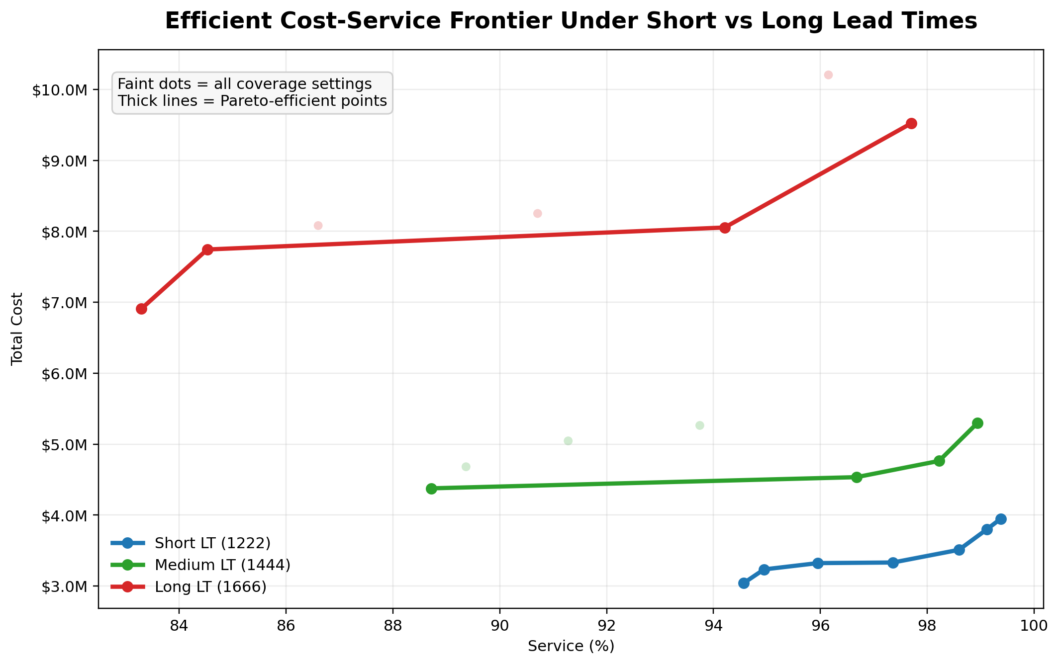
The strategic result is that the three regimes do not sit on one shared trade-off curve6. They form different possibility spaces. A long lead-time network can improve service, but it does so from a structurally higher cost base.
That matters because optimization inside a slow regime has a ceiling. The long profile can buy its way toward higher service, but the frontier says it is paying for time before it is paying for performance.
Business recommendation: treat lead-time reduction as a structural improvement program, not as a local inventory tuning exercise.
2. Capacity Is Not the Main Escape Route
The next chart tests whether capacity can compensate for slow time. Each cell shows the coverage required to reach 95% service for a specific lead-time profile and capacity multiplier.
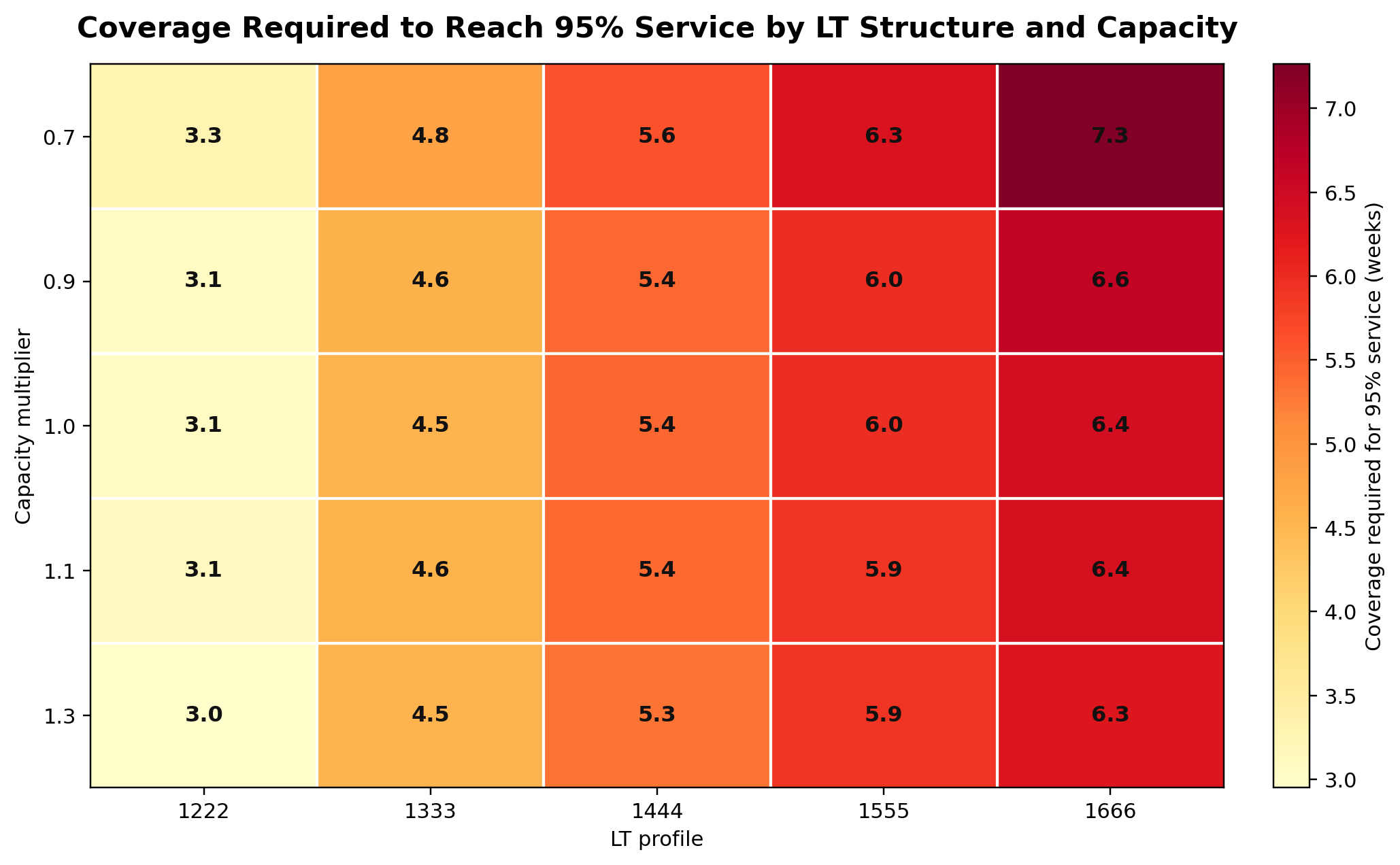
The heatmap shows that capacity helps, but not enough to change the strategic answer. Required coverage changes sharply from left to right as lead-time profiles lengthen. It changes much less from top to bottom as capacity increases.
- At the shortest profile, required coverage is roughly 3.0 to 3.3 weeks across capacity levels.
- At the longest profile, required coverage remains around 6.3 to 7.3 weeks even with more capacity.
- Moving from low to high capacity trims the requirement, but shortening lead time changes the whole requirement band.
The operational read is simple: capacity is a useful local relief valve, but it does not reset the economics the way lead-time compression does.
Business recommendation: use capacity expansion selectively; prioritize lead-time reduction when the goal is to lower inventory requirements.
3. The Cost of Time Lands Upstream
The third chart compares networks that reach the same 95% service level but carry very different cost structures. The bars split interpreted total cost across retailer, distributor, manufacturer, and supplier stages.
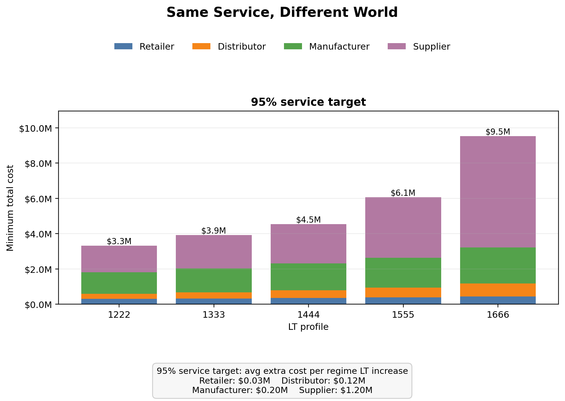
This explains why the lead-time problem is easy to miss if the network is judged only from the customer-facing service number. Even when every profile is read at the same 95% service level, longer lead-time profiles create much higher interpreted total cost. The retailer does not absorb the main shock; the burden moves upstream, with the supplier carrying the largest increase.
- At 95% service, total interpreted cost rises from about 1.5M in the shortest profile to about 7.2M in the longest profile.
- The retailer and distributor remain comparatively stable, while the supplier-side cost expands most visibly as lead times lengthen.
This turns lead-time reduction into a value-chain problem. A slower upstream structure can leave downstream service looking acceptable while concentrating operational pressure on supplier-facing stages.
In practice, that pressure is not passively absorbed. It is redistributed through commercial mechanisms such as pricing, order constraints, and commitment structures. When lead time increases, the cost must be carried somewhere in the system.
In this simulation, that burden appears upstream by construction. The model represents a single-network view and does not include the contractual feedback loops that would shift part of the cost back downstream. The result should therefore be read as a map of where operational pressure accumulates, not as a claim about how cost is ultimately shared in real supply chains.
Business recommendation: treat supplier responsiveness as part of the economic design of the network, not as a side negotiation after the inventory policy is chosen.
4. One Inventory Rule Will Not Fit Every Demand Family
The final chart adds the segmentation layer. It shows the coverage required for each demand family as lead-time profiles move from short to long.
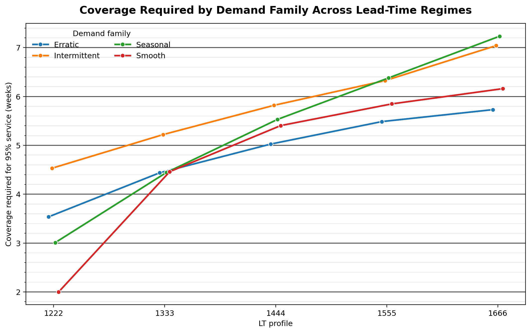
Lead-time reduction should not be applied as a generic program with the same expected return everywhere. Demand families react differently as lead times stretch.
- Seasonal and intermittent demand require the most coverage under long lead-time profiles, rising to roughly 7 weeks or more.
- Smooth demand starts from the lowest coverage need and remains less exposed, though it still rises as lead time lengthens.
- Erratic demand grows more moderately than seasonal and intermittent demand in this experiment.
That creates a practical prioritization rule: start lead-time reduction where the coverage burden is most sensitive to delay, then use differentiated coverage policies rather than forcing one buffer target across the portfolio.
Business recommendation: prioritize lead-time reduction for seasonal and intermittent SKUs, where delay creates the steepest coverage requirement.
Decision Framework
The case points to a different order of operations than a standard inventory review. Inventory coverage is still needed, and capacity can still matter, but both are downstream responses to the network's time structure.
| Decision area | What the analysis shows | Action implied |
|---|---|---|
| Lead-time reduction | Lead time shifts the whole cost-service frontier and drives the largest change in required coverage. | Treat speed as a strategic lever, not only a supplier KPI. |
| Capacity expansion | Capacity lowers coverage needs at the margin but does not escape the long lead-time regime. | Use capacity to relieve bottlenecks after the time problem is understood. |
| Supplier collaboration | Long lead times push cost upstream, especially into supplier and manufacturer stages. | Work with suppliers on responsiveness, not only unit price. |
| SKU prioritization | Seasonal and intermittent families show the highest coverage burden under long lead times. | Target those families first for lead-time and planning-policy redesign. |
Key Takeaways
- Service level is the visible outcome; lead-time structure is the hidden constraint shaping the cost of that outcome.
- Inventory coverage protects service, but high coverage requirements are often evidence of a slow network rather than proof that more stock is the best answer.
- Capacity expansion is useful when it relieves a specific bottleneck, but it does not move the cost-service frontier as strongly as lead-time reduction.
- The cost of long lead times accumulates upstream, so supplier collaboration should focus on responsiveness as well as price.
- Lead-time reduction should be prioritized by demand family, with seasonal and intermittent SKUs offering the clearest inventory-saving opportunity in this experiment.
Terminology Notes
- Four-stage supply network: the simulated supply chain has four connected stages: Retailer, Distributor, Manufacturer, and Supplier.
- Coverage: weeks of inventory protection. More coverage means more buffer, but also more cash and cost tied up in the system.
- Lead-time profile: a four-digit scenario code for stage delays. The digits are ordered downstream to upstream: distributor-to-retailer, manufacturer-to-distributor, supplier-to-manufacturer, and supplier raw-material production. Profile 1222 means 1, 2, 2, and 2 weeks; profile 1666 means 1, 6, 6, and 6 weeks.
- Demand family: a group of SKUs that behave similarly, such as steady, seasonal, intermittent, or highly volatile demand.
- Capacity level: the production capacity setting tested in the simulation, expressed as a multiplier such as 0.7 for constrained capacity or 1.3 for expanded capacity.
- Cost-service trade-off curve: the best available balance between total cost and service level. Points above the efficient frontier are worse options because they cost more for the same or lower service.
Method Notes and Limits
This is a calibrated simulation case, not a plug-and-play operating policy. The purpose is to show how lead-time structure changes the economics of service and where a planning team should look before adding inventory or capacity.
- Demand, cost parameters, lead-time assumptions, and capacity calibration are synthetic and should be re-estimated for operational use.
- The lead-time profile labels are scenario codes used for comparison, not literal supplier contracts.
- The page summarizes the main portfolio signal; operational deployment would require SKU-level service targets, supplier constraints, and implementation cost estimates.